Introduction

Accurate and efficient methods for pricing and hedging financial derivatives is critical in many financial applications. Many derivatives have well developed mathematical models, but the models do not have a closed form solution. The pricing of American put options is a case in point.

This project explores the different numerical methods for solving European, and, most importantly, American put options derived from the well-known Black-Scholes equation. Mainly, we focus on both accuracy and efficiency of each algorithm.

Approach

The Black-Scholes equation is given by: \({\partial V \over \partial t} + {1\over 2} \sigma^2 S^2 {\partial^2 f \over \partial S^2} + r S {\partial V \over \partial S} - rV = 0\)

For European put options, we transform the problem to a diffusion equation and develop mesh approximation to numerically solve the partial differential equation. Take \(S = E e^x, t = T - \tau / {1/2} \sigma^2, V = E v(x, \tau), k = r / {1\over 2} \sigma^2\)

Also, let \(v = e^{-{1\over 2}(k-1)x - {1\over 4} (k+1)^2\tau} u(x, \tau)\)

The Black-Scholes equation now becomes \({\partial u \over \partial \tau } = {\partial^2 u \over \partial x^2} \ {for} -\infty < x< \infty, \tau > 0.\)

To reach a finite mesh approximation, we cut the $(x, \tau)$ domain into a finite mesh with tiny space. Denote $u_n^m = u(n\delta x, m\delta \tau)$. By forward difference approximation of $\partial u \over \partial x$ and $\partial u \over \partial \tau$, we have \({u_n^{m+1} - u_n^m \over \delta \tau} + O(\delta \tau) = {u_{n+1}^m - 2 u_n^m + u_{n-1}^m \over (\delta x)^2 } + O( (\delta x)^2)\) and backward difference approximation: \({u_n^{m} - u_n^{m-1} \over \delta \tau} + O(\delta \tau) = {u_{n+1}^m - 2 u_n^m + u_{n-1}^m \over (\delta x)^2 } + O( (\delta x)^2)\)

If we take $\alpha = {\delta \tau \over (\delta x)^2}$, the forward and backward difference approximation will be: \(u_n^{m+1} = \alpha u_{n+1}^{m} + (1-2 \alpha) u_n^{m} + \alpha u_{n-1}^{m}\) and \(u_n^{m-1} = -\alpha u_{n-1}^{m} + (1+2 \alpha) u_n^{m} - \alpha u_{n-1}^{m}.\)

Based on either forward or backward difference approximation, several algorithms can be developed numerically to solve the diffusion equation. In this project, we examine only the Explicit Forward Method, Implicit LU Method, Implicit SOR Method, Crank-Nicolson LU Method and Crank-Nicolson SOR Method. The detailed explanation and Pseudocode of each method is listed in [1]. Briefly, the difference between the LU and SOR methods is that the LU method uses LU matrix factorization to solve a large system of equations, whereas the SOR method uses iterative guesses to get an approximated value under certain error tolerance. The difference between the Implicit and Crank-Nicolson Method is that the Crank-Nicolson Method applies both forward and backward difference approximation to get a lower error order.

For American put options, the idea of the linear complementary problem is used to solve the free boundary condition in the partial differential equation. Now, we need to solve the following relationship:

\({\partial u \over \partial \tau} = {\partial^2 u \over \partial x^2} \ for\ x > x_f(\tau),\ else\ {\partial u \over \partial \tau} > {\partial^2 u \over \partial x^2}\) \(u(x, \tau) = g(x, \tau) \ for\ x \leq x_f(\tau),\ else\ u(x, \tau) > g(x, \tau)\)

where $x_f(\tau)$ is the free boundary in the linear complementary problem and $g(x, \tau)$ is the payoff function:

In order to solve this problem, we need to apply the PSOR method, which is a slight modification based on SOR. The derivation and Pseudocode are also listed in [1]. Briefly, in PSOR, at each time step, if the estimated value is below the payoff function, we need to use the payoff value instead of the estimated value. This is because the nature of American options is such that the value at the time before maturity is always larger or equal to the value at maturity.

Analysis

European Put Options

In this project, we mainly focus on the accuracy of each method. For European put options, as we have a closed form of solution, the Black-Scholes formula, error of each method is very easy to compute. Figure 1 is generated from Implicit LU Method as an example (the plots for other methods are omitted here).

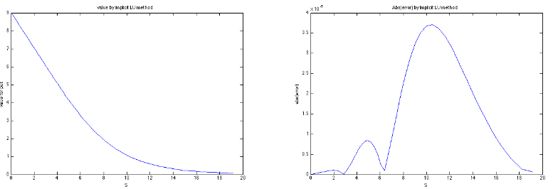
Figure 1: Parameters of the European put option: $E = 10, r = 0.1, \sigma = 0.4, T-t = 1$. The left is the estimated value of the option while the right is the absolute value of the error from estimating this option using the Crank-Nicolson LU Method.

Note that in general, the magnitude of error compared to the Black-Scholes formula is less than 4e-3, which is sufficiently small for most applications. Also, the error increases as S approaches the exercise price $E = 10$. This is due to the fact that there is a saddle point around $S = 10$. When $S$ is much smaller than 10, the result is approximately linear. If $S$ is much larger than 10, the value converges to 0. In both cases, they leave little room for the approximation. Thus, the induced error is quite small. However, around $S = 10$, we have a transition from one linear line to another. In this case, the approximation is used heavily. Therefore, we observe a larger error around $S = 10$.

Also, for the Implicit Method, the error is of order $O(\delta \tau) + O((\delta x)^2)$(proven in [1]). To better check this important behavior, we can plot error versus $(\delta \tau)$ and $(\delta x)^2$ respectively (Figure 2).

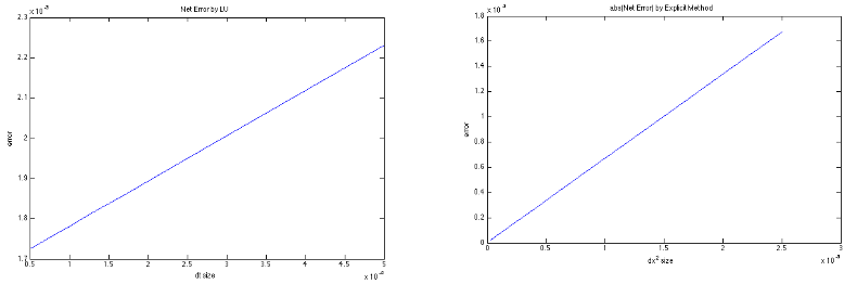
Figure 2: Parameters of the European put option: $E = 10, r = 0.1, \sigma = 0.4, T-t = 1$. The left is plotted by error versus dt while the right is by error versus $dx^2$.

American Put Options

![Parameters of the American put option: $E = 10, r = 0.1, \sigma = 0.4, T-t = 1$. The left is the estimated value of the option before maturity(in blue) where the right is the error ratio plotted with respect to S. $S_f(t)$ is cawidth=”16cm”}

For American put options, we do not have a closed form solution to compare. However, there are two general ways to examine the accuracy of our PSOR algorithm. Firstly, we can plot the estimated value and compare it visually to the European put option with same parameters. By the nature of the linear complementary problem, the value would be the same as the payoff function before the free boundary $S_f(t)$ and larger than that after $S_f(t)$. By the smoothness assumption of the linear complementary problem, at $S_f(t)$, the function should be tangent to the payoff function. These behaviours can be nicely checked in Figure 3(left).

Secondly, note that if we change the size of $\delta x$ and $\delta \tau$ proportionally, the error should also change proportionally. As PSOR is modified from the Crank-Nicolson Method, the order of error is approximately $O((\delta \tau)^2) + O((\delta x)^2)$. Pick $\delta x_1$ and $\delta \tau _1$. Let \(\delta x_2 = {1\over 2} \delta x_1,\ \delta \tau _2 = {1\over 2} \delta \tau_1\) \(\delta x_3 = {1\over 4} \delta x_1,\ \delta \tau _3 = {1\over 4} \delta \tau_1\) Then \(P_1 \approx P + a (\delta \tau_1)^2 + b(\delta x_1)^2\) \(P_2 \approx P + a (\delta \tau_2)^2 + b(\delta x_2)^2 = P+ {1\over 4}(a (\delta \tau_1)^2 + b(\delta x_1)^2)\) \(P_3 \approx P + a (\delta \tau_3)^2 + b(\delta x_3)^2 = P + {1\over 16}(a (\delta \tau_1)^2 + b(\delta x_1)^2)\) Then, subtracting, \(P_1 - P_2 = {3\over 4}(a (\delta \tau_1)^2 + b(\delta x_1)^2)\) \(P_2 - P_3 = {3\over 16}(a (\delta \tau_1)^2 + b(\delta x_1)^2).\)

Figure 3: Parameters of the American put option: $E = 10, r = 0.1, \sigma = 0.4, T-t = 1$. The left is the estimated value of the option before maturity(in blue) where the right is the error ratio plotted with respect to S. $S_f(t)$ is calculated to be approximately 7.408.

Therefore we should have the following relationship: \(P_1 - P_2 \approx 4 (P_2 - P_3).\)

The ratio of ${P_1 - P_2} \over P_2 - P_3$ is plotted in Figure 3 (right). Note that only the ratio near $S = 10$ part is of our interest. When $S$ is smaller than the free boundary $S_f(t) = 7.408$, the error ratio randomly picks $0$ or $NaN$. This is because before free boundary, the estimated values are the same as in the payoff function. Therefore, most of the time, the denominator is 0 and the ratio is undefined. As $S$ increases, the estimated value will converge to 0 so quickly that the approximation algorithm is not deeply used. The ratio will again be uninterpretable.

Conclusion

Overall, this project examines different methods for pricing European put options with the PSOR Method for American put options. For the European put option part, the Crank-Nicolson Method provides a more precise estimation. When talking about efficiency, the LU Method is much faster than the SOR Method because the SOR-solver function needs to iterate until convergence at each time step. For American options, in practice, the PSOR Method computes very slowly as it also must iterate until convergence. By adjusting the over-relaxation parameter, the runtime of computing convergence is optimized.

The underlying assumption for the pricing problem is quite simple. We ignore the effect of transaction fee, dividends, etc. However, these advanced assumptions can be included by further modifications based on these algorithms. Moreover, we can also price another type of option by changing the payoff function. These topics are beyond the scope of our discussion here.

The major difficulty for this project is understanding how to transform the Black-Scholes equation to a numerically solvable problem. I believe the value of this idea is beyond just pricing options. This project may inspire me in the future whenever I need to apply numerical approaches to the encountered problem.

References

1. Howison, S., Dewynne, J., Wilmoot, P. The mathematicas of financial derivatives: A student introduction. 1995