1 Introduction
This project explores Partial Differential Equation (PDE)
discretization methods for discontinuous coefficient PDEs, with application to a mathematical model simulating the invasion of brain cancer (glioma). This model involves a PDE with discontinuous diffusion coefficient due to the heterogeneous nature of the brain, consisting of white and grey matters.
PDEs are ubiquitous in modeling many physical phenomena. Phenomena that involve diffusion (scattering) and reaction (e.g. proliferation) are often modelled by the so-called $reaction-diffusion$ PDEs. Such PDEs are pertinent to cancer growth, as the latter involves scattering and proliferation of cancerous cells.
Physical problems that involve unknown quantities that are evolving in time (and vary along spacial dimensions) are modelled by time-dependent PDEs. These PDEs, together with equations describing the initial state (referred to as $initial$ $conditions$), and equations describing the boundary behaviour of the unknown (referred to as $boundary$ $conditions$), form an $Initial$ $Value$ $Problem$ (IVP). On the other hand, if the unknown quantities vary only along spacial dimensions, the PDEs together with boundary conditions form a $Boundary$ $Value$ $Problem$ (BVP).
Often, PDEs cannot be solved by analytic methods. In such cases, numerical methods are employed for the PDE solution. The numerical solution involves two main steps: the conversion of the continuous problem into a set of discrete algebraic equations, referred to as $discretization$, and the solution of the arising set of equations (often a linear system of equations), which results in discrete approximate values of the unknown quantities or other related discrete values. The size of the system of equations depends on the number of discrete points/data ($discretization points$) taken in the domain of the problem. The discretization method is critical for the accuracy of the solution, as well as for the correctness of the solution, in the sense of satisfying any special conditions or constraints arising from the problem. A discretization method should $converge$, in the sense of the approximate solution values converging to the exact ones, as the number of discretization points increases. Faster convergence (i.e. a higher $order$ $of$ $convergence$) is desirable.
The partial derivatives occurring in a PDE often appear with coefficient functions. Standard numerical PDE methods normally assume continuous coefficient functions. However, when these discretization methods are applied to a discontinuous coefficient PDE, convergence of the approximate solution, as the number of discretization points increases, is not guaranteed. Studying numerical methods for PDEs with discontinuous coefficients is pertinent to brain cancer growth, as it is known that the brain consists mainly of grey and white matter, and the diffusion rate (represented by a coefficient function) is higher in the white than in the grey matter.
In previous studies, some researchers formulated Hermite spline collocation methods for discontinuous diffusion PDEs [1][2], using a clever adjustment of the basis functions to satisfy certain constraints resulting from the discontinuity of the coefficient. In [3], quadratic spline collocation methods are used, and in [4], adaptive Hermite spline collocation is formulated for the same problem, with a clever approximation of the discontinuous diffusion coefficient. In all these works, the expected (fourth) order of convergence is obtained.
Finite Difference (FD) methods (approximating derivatives by linear combinations of discrete function values) are popular and flexible discretization methods for PDEs. We propose two approaches to adjust the standard FD methods, so that the numerical solution satisfies the constraints resulting from the discontinuity of the coefficient, and converges with the expected order of convergence.
In Section 2, we present the problems considered. In Section 3, we describe the numerical methods developed, in particular regarding discontinuous diffusion, and in Section 4, we demonstrate results from numerical experiments that show the effectiveness of our methods. We conclude in Section 5.
2 Discontinuous Diffusion PDE
The PDE under consideration is the Reaction-Diffusion PDE in one spatial dimension \begin{equation} \label{eq:IVP} u_t = (d(x)u_x)_x + \rho u + f(x, t) \equiv \mathcal{L}u + f(x, t), ~ \mbox{in} ~ [a, b] \times (0, t_f), (1) \end{equation} where $u(x,t)$ is unknown quantity dependent on $x$ (spatial coordinate) and $t$ (time), which diffuses (spreads around) with diffusion coefficient $d(x)$ and grows (proliferates or reacts) with coefficient $\rho$. Given the initial (at time $t = 0$) state of $u$, and some conditions at the boundary of the spatial domain, we want to predict the state at some given final time $t = t_f$. PDE (1), together with these initial and boundary conditions, forms an IVP.
(In most realistic problems, the forcing term $f(x, t)$ is equal to zero, but we may set it to non-zero for the purpose of certain numerical experiments.)
In the mathematical model for the density of tumoral cells in the brain of a patient, considered in [5], the non-homogeneity of brain (grey and white matter, reflected in the discontinuity of the diffusion coefficient) is modelled as
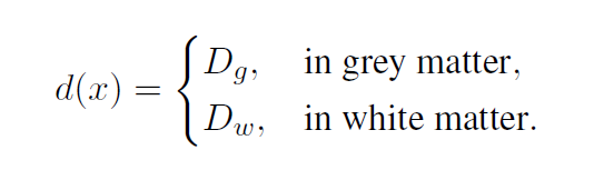
For simplicity, the two values of the diffusion coefficient in the white and grey matter are set as follows: Let $D_w=1$ and $D_g = \gamma$ where $\gamma = \frac{D_g}{D_w} < 1$ is a parameter chosen by the user. Assume, for simplicity, two interfaces: from left to right, $w_1$ (grey to white) and $w_2$ (white to grey). See Figure 1.
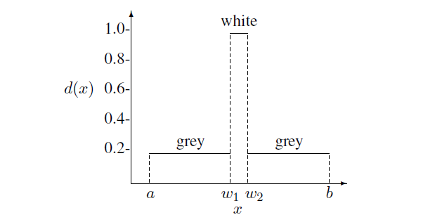
Figure 1: diffusion coefficient $d(x)$ as it varies with $x$.
The presence of the discontinuity in the diffusion coefficient results in a certain type of (dis-)continuity conditions across interfaces modelled as
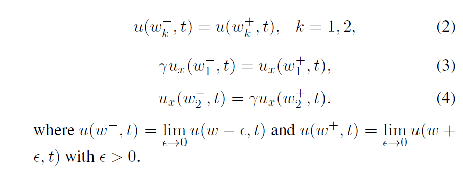
Since the discontinuities occur along the space dimension, we also consider a BVP, described by the PDE
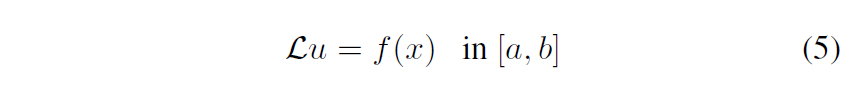
where the solution $u(x)$ satisfies (dis-)continuity conditions similar to (1)-(2), and boundary conditions similar to those the solution of (1) satisfies.
The space discretization techniques are easier to describe for the BVP than for the IVP. For this reason, we focus on the description of the space discretization techniques for the BVP in detail, and these techniques can be applied to the IVP.
3 Numerical Methods
consider the space discretization of PDE (5). We discretize the spatial domain as shown in Figure 2.
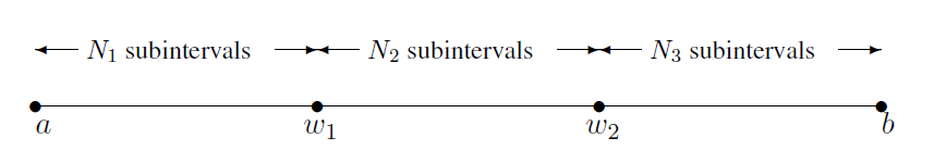
Figure 2: Domain discretization
For simplicity, we use uniform discretization. Let $x_0=a$, $x_i = a+ih_x~(i=1,\dots, N)$, $N=N_1+N_2+N_3$ and $h_x=\frac{b-a}{N}$. Also for simplicity, assume that $w_1 = x_{N_1} = x_k, w_2=x_{N_1+N_2}$ and $u(x_i)$ = $u_i$. Note that $N$ is the total number of subintervals and $N+1$ the total number of discretization points including boundary.
Two approaches were developed in the project to deal with discontinuous diffusion.
$Approach$ $1$
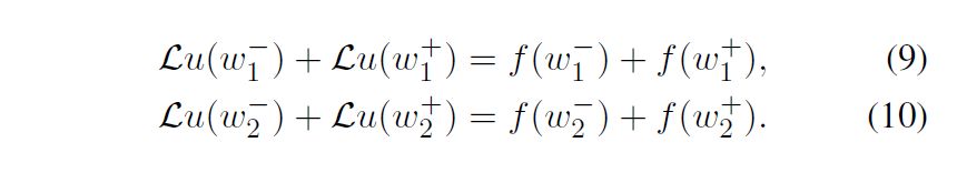
We treat the PDE as multi-domain problem with individual respective approximations for each subdomain, and use the interface conditions as “boundary” conditions for the subdomain problems. Specifically, the equations used at the interface points are:
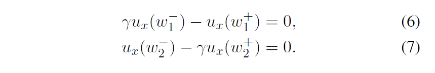
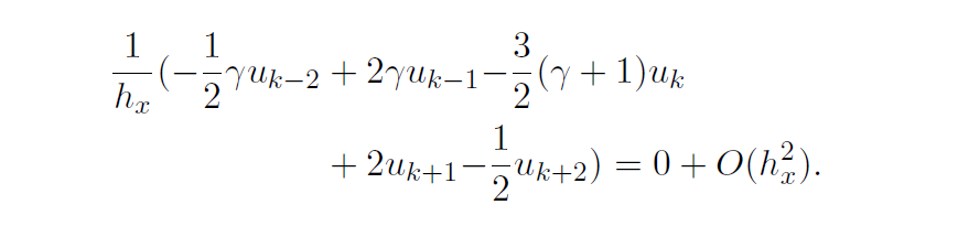
Discretizing each term of equation (6) by one-sided FDs and taking into account (2) results in
Note that, for non-interface points, we use the standard equations
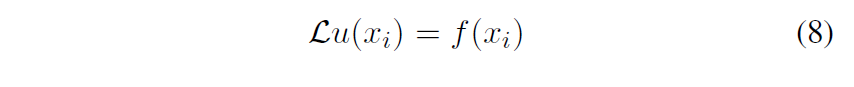
discretized by standard second-order FDs.
$Approach$ $2$
For all non-interface points, we use the same space discretization as in the first approach. For the interface points, we establish equations to relate %the limits of the functional and forcing terms from both sides the limits of the PDE terms from both sides of the interface point. The equations used at the interface points are:
To discretize equation (9), we form one-sided stencils that involve $u_{xx}$ and $u_x$, take a linear combination of them so that the $u_x$ terms are cancelled using the discontinuity condition (3), while condition (2) is also taken into account, then add appropriate terms to form $\mathcal{L}u(w_1^-)$ and $\mathcal{L}u(w_1^+)$. Then we get
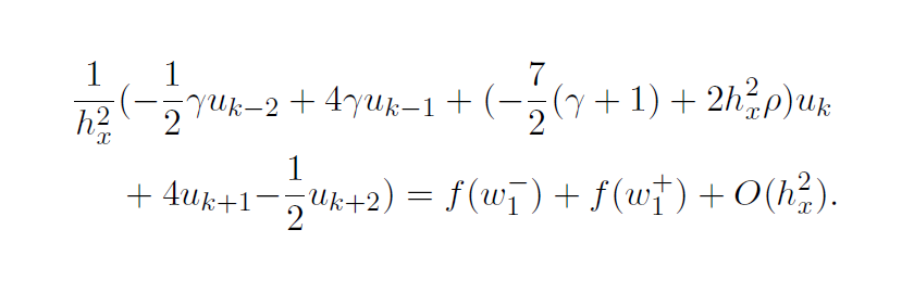
In the above relation, the term $f(w_1^-) + f(w_1^+)$ is approximated by $f(w_1-\epsilon) + f(w_1+\epsilon)$, for a suitably small $\epsilon > 0$. Relation (10) is discretized similarly.
Following a similar derivation, the proposed space discretization methods can be extended to fourth-order accuracy (error in spatial discretization is $O(h_x^4)$), for both the interface and non-interface points.
Coming back to (1), for the time discretization, we adopt the standard Crank-Nicolson timestepping scheme, with $\Delta t \propto h_x$, and, for the space discretization, the techniques we described for the PDE (5).
4 Numerical Results
We first test the proposed space discretization schemes on a BVP, then extend them to IVPs. In all problems, we used $\gamma = 0.20$, $\rho = 1$, $a = -5$ and $b = -a$. In Problems 1 and 2, $w_1 = -0.5$, $w_2 = -w_1$, and in Problem 3, $w_1 = 0$ and $w_2 = 2$.
In Problem 1, we pick a function $u$ that satisfies the interface conditions and take its gradients as defined in $\mathcal{L}u$ to form the non-zero forcing term $f(x)$. Then, Problem 1 is a BVP with a known solution, guaranteed to satisfy the interface conditions. When we apply each of our approaches to Problem 1, we obtain respective approximate solutions that can be compared to the (known) exact one. Such a problem can be used as a benchmark to evaluate the accuracy of our computed approximate solutions.
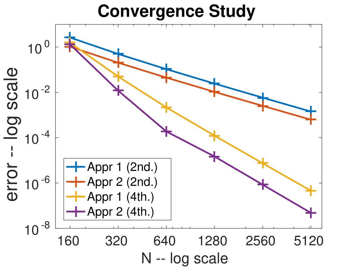
Figure 3: Plot of error versus the total number of subintervals $N$ for Problem 1. For Approach 2, $\epsilon = 10^{-10}$.
In Figure 3,the error of the computed solution decreases in the expected order: when the number of discretization points is doubled, the error becomes approximately 4 times smaller for the second-order method and 16 times smaller for the fourth-order method. The slope of the error plots indicates the (negative) order of convergence.
Problem 2 is an IVP with exact solution known, and a non-zero forcing term $f(x,t)$ formed according to PDE (1). The solution satisfies the interface conditions at all points in time and the state of $u$ at $t=0$ is given as the initial condition. Again, as in Problem 1, we compute approximate solutions by our approaches and compare them to the (known) exact one.
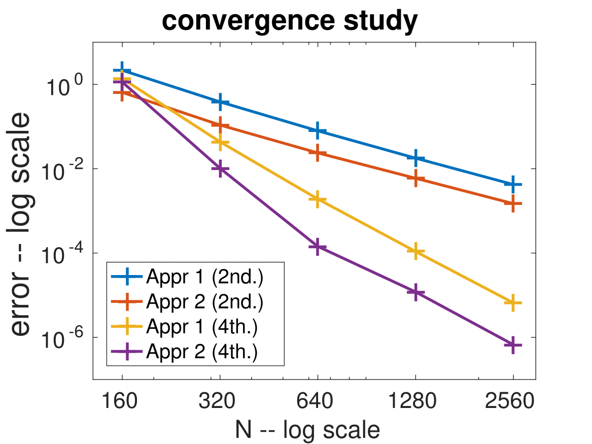
Figure 4: Plot of maximum error among all points in time versus $N$ for Problem 2. For Approach 2, $\epsilon = 10^{-10}$.
In Figure 4, the error decreasing trend is similar to the BVP case. The convergence results match the expected ones.
Problem 3 is an IVP with exact solution unknown, and a zero forcing term $f(x,t)$. The initial condition satisfies the interface conditions.
While, as mentioned in the Introduction, other researchers managed to obtain fourth-order methods for the same problem, we did this by employing the simpler, more flexible and more widely used Finite Difference methods.
Note that both the proposed methods can be generalized to more interfaces, and to non-uniform grid discretizations. We also plan to consider adaptive FD methods and extension to multiple space dimensions.
Acknowledgement
I would like to express my sincere gratitude to my supervisor Christina Christara for her valuable guidance and kindly encouragement, and to the University of Toronto Excellence Award (UTEA) program for funding the project.
References
-
M. G. Papadomanolaki and Y. G. Saridakis, “Collocation with discontinuous Hermite elements for a tumour invasion model with heterogeneous diffusion in 1+1 dimensions, ”in Numerical Analysis conference, NumAn2010, pp. 214–223, September 2010.
-
I. E. Athanasakis, M. G. Papadomanolaki, E. P. Pa-padopoulou, and Y. G. Saridakis, “Discontinuous Hermitecollocation and diagonally implicit RK3 for a brain tumour invasion model,” in World Congress on Engineering WCE, Vol 1, pp. 1–6, July 2013.
-
C. Christara, “Numerical methods for discontinuous diffusion parabolic PDEs with application to brain tumor growth, oral presentation,” in Canadian Applied and Industrial Mathematics Society conference, June 2014. oralpresenation.
-
C. Christara, “Adaptive and non-adaptive spline collocation methods for pdes with discontinuous coefficients: application to brain cancer growth,” in Canadian Applied and Industrial Mathematics Society conference, July 2016. oralpresenation.
-
K. R. Swanson, E. Alvord, and J. Murray, “A quantitativemodel for differential motility of gliomas in grey and white matter,”Cell proliferation, vol. 33, no. 5,pp. 317–329,2000.