Introduction: semantic maps and case study
Linguistic typology is a subfield of linguistics concerned with cross-linguistic variation in language structure. Not all logically possible variations occur in language, and in fact, there are strong preferences for certain ways of organizing linguistic structures over others. In this project, we investigate visual representations of language patterns through a case study on time phrases like in 1980 and on Monday. Haspelmath divides these so-called simultaneous location temporal adverbials into six categories that hold across languages [1]: Hour (at 6 o’clock), Day Part (in the morning), Day (on Monday), Month (in May), Season (in Winter), and Year (in 1980). Time phrases are of interest to typologists because they show significant variation between languages. For example, English uses the same preposition for Year, Season, and Month (in 1980, in Winter, in May); Swedish uses different prepositions for each (under 1980, p vintern, i maj); and Tagalog groups Month and Season together, but not Year (nang 1980, sa kalamigan, sa Mayo).
We can study this variation by considering groupings of semantic categories (here, the six time categories) that are associated with a single preposition in a language. For example, in English, there is a grouping for the categories Day Part, Season, Year, and Month, since these are all associated with the preposition in. Variation in how languages combine categories into groupings is not arbitrary. For example, it is very common for languages to have a preposition used only for Hour, but no languages in our data have a Month-Hour grouping (i.e., using the same preposition for both). Typologists aim to reveal and understand these patterns.
One way of formalizing this information is a semantic map, a graph in which semantic categories are represented by nodes, and groupings of categories form connected sets of nodes in the graph (see Fig. 1-3). That is, a set of categories that are associated with a single word forms a set of nodes that are all connected, be it directly or indirectly. The goal is to choose the edges for a semantic map such that all groupings in all languages under consideration form said connected sets of nodes. Thus, the map represents the cross-linguistically observed constraints on those semantic groupings. This means that categories in the same grouping for some language should either be connected by an edge (like Year and Month in the in grouping in Fig. 1) or connected through a series of nodes also in the grouping (like Day Part and Year in the in grouping in Fig. 1); the latter indicates that it would not be expected for Day Part and Year to share a preposition in any language without Season also using the same preposition.
Traditionally, semantic maps were hand-drawn based on cross-linguistic data, but recently researchers have begun computing them. Here, we propose new methods for inferring and evaluating semantic maps, and explore them through our case study on time phrases.
Inferring semantic maps
Regier and colleagues present a computational method for inferring semantic map graphs [2]. This is done by maximizing a connectedness score, which measures how many groupings in the data correspond to connected regions in the graph. Maximizing the connectedness score creates graphs that account for the groupings for each language in the data. The algorithm in Regier’s paper works as follows: (1) start with a graph with no edges, (2) look through all possible edges and add the edge that results in the graph with the highest connectedness score, (3) repeat step 2 until all groupings form connected subgraphs.
A limitation of this approach is that it results in highly connected graphs if there is a lot of variation. While highly connected graphs are more complete in representing groupings that exist in the data, they also predict many possible groupings that are not found in any of the world’s languages. Simpler maps may not account for the diversity of all groupings, but also do not overpredict possible groupings. These aspects of the graph/data relationship create tension with each other, and graph-inferring algorithms need to find a balance between them. To complement the connectedness score, we propose the fit score, which is equal to the fraction of subgraphs in a semantic map that correspond to a grouping in one of the languages in a data set. Where the connectedness score captures the extent to which groupings in the data are connected in the graph, the fit score captures the extent to which the connected regions in the graph correspond to groupings in the data.
We use the harmonic mean of these two scores, or the combined score, as an objective function. Like the algorithm used in the Regier paper, our algorithm iteratively adds nodes maximizing the combined score objective function. This algorithm stops adding new edges when doing so no longer increases the graph’s combined score.
Data sets
Two data sets were used in this case study. The Haspelmath data set [1] was manually constructed based on dictionaries, corpus data, and grammars written by linguists. The auto data set was constructed for this project using the Bible corpus [3]. For the auto data set, a word alignment model [4] was used to extract phrase translations from a parallel corpus, after which the words per semantic category were identified manually. The Haspelmath data set contains data on 53 languages, and the auto data set has data on 23 languages. Both data sets have a higher proportion of Indo-European languages but are otherwise genetically and geographically diverse.
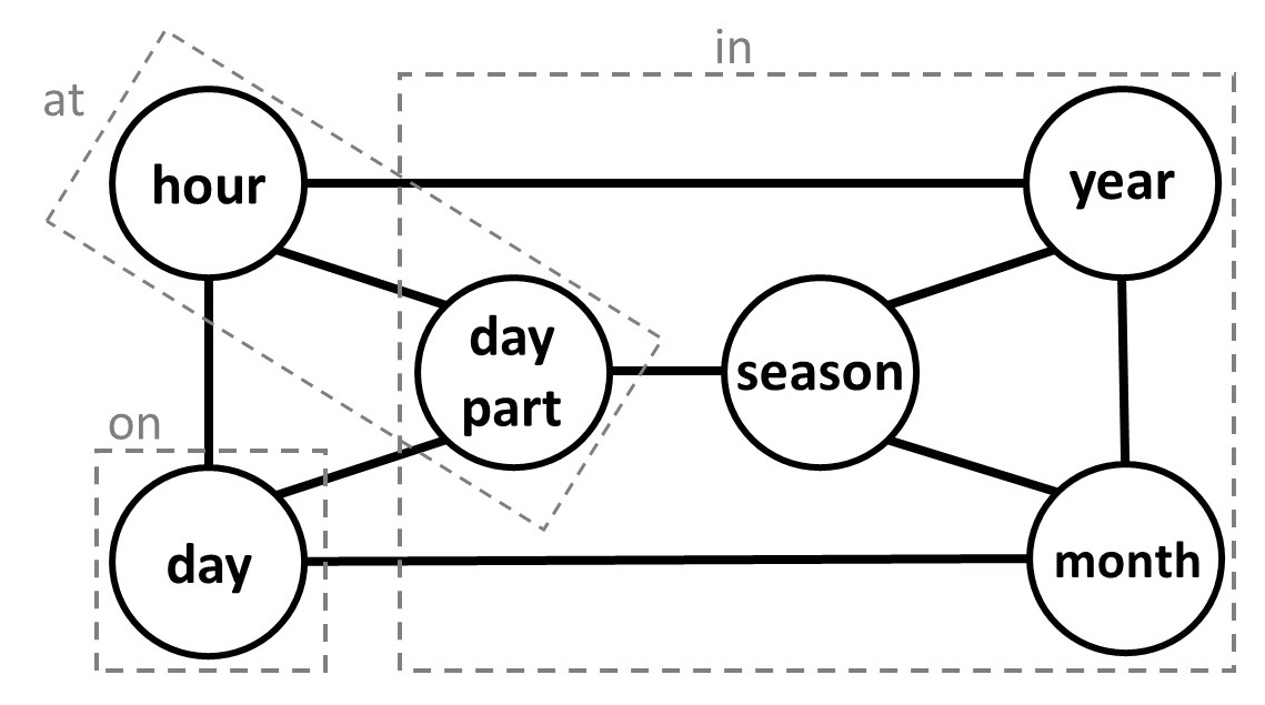
Figure 1: Map manually created by Haspelmath for his data.This diagram is labelled with the groupings for English.
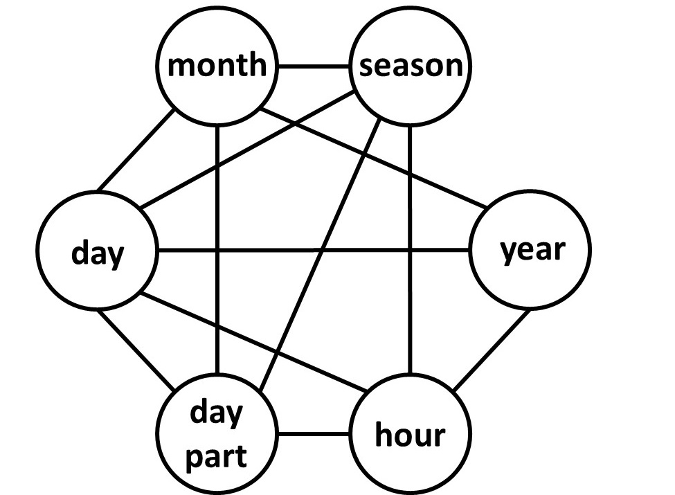
Figure 2: Connectedness map automatically constructed using Haspelmath data andconnectedness objective function.
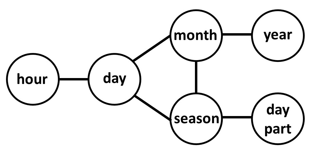
Figure 3: Combined map automatically constructed using Haspelmath data andcombined objective function.
Results
Here, we compare the results for Haspelmath’s data across 3 semantic maps: a manually drawn map, a map inferred using the connectedness objective function, and a map inferred using our combined objective function. (The results achieved by the auto data for the two objective functions were similar.) In comparing the manual map (Fig. 1) to the connectedness map (Fig. 2), the manual map has 11 groupings in the data not connected in the map, where the connectedness map has none. The connectedness map, however, predicts 19 groupings that are not attested in any languages. In contrast, the combined map predicts only 3 unattested groupings, but has 31 groupings in the data not connected in the graph (Fig. 3). The combined objective function provides a different, interesting perspective by producing a much simpler visualization while minimizing the amount of non-predicted but attested cases.
References
-
M. Haspelmath. From Space to Time: Temporal Adverbials in the World’s Languages. Lincom Europa, Munich and Newcastle, 1997.
-
A. Majid T. Regier, N. Khetarpal. Inferring semantic maps. Linguistic Typology, 17:89–105, 2013.
-
M. Cysouw T. Mayer. Creating a massively parallel bible corpus. Oceania, 135(273):40, 2014
-
D. Klein P. Liang, B. Taskar. Alignment by agreement. Proceedings of the mainconference on Human Language Technology Conference of the North AmericanChapter of the Association of Computational Linguistics, pages 104–111, 2006.